16. DOA & Beamforming

In this chapter we cover the concepts of beamforming, direction-of-arrival (DOA), and phased arrays in general. Techniques such as Capon and MUSIC are discussed, using Python simulation examples. We cover beamforming vs. DOA, and go through the two different types of phased arrays (Passive electronically scanned array or PESA and Active electronically scanned array or AESA).

Overview and Terminology

A phased array, a.k.a. electronically steered array, is an array of antennas that can be used on the transmit or receive side to form beams in one or more desired directions. They are used in both communications and radar, and you’ll find them on the ground, airborne, and on satellites.

Phased arrays can be broken down into three types:

1. Passive electronically scanned array (PESA), a.k.a. analog or traditional phased arrays, where analog phase shifters are used to steer the beam. On the receive side, all elements are summed after phase shifting (and optionally, adjustable gain) and turned into a signal channel which is downconverted and received. On the transmit side the inverse takes place; a single digital signal is outputted from the digital side, and on the analog side phase shifters and gain stages are used to produce the output going to each antenna. These digital phase shifters will have a limited number of bits of resolution, and control latency.
2. Active electronically scanned array (AESA), a.k.a. fully digital arrays, where every single element has its own RF front end, and the beamforming is done entirely in the digital domain. This is the most expensive approach, as RF components are expensive, but it provides much more flexibility and speed than PESAs. Digital arrays are popular with SDRs, although the number of receive or transmit channels of the SDR limits the number of elements in your array.
3. Hybrid array, which consists of subarrays that individually resemble PESAs, where each subarray has its own RF front end just like with AESAs. This is the most common approach for modern phased arrays, as it provides the best of both worlds.

An example of each of the types is shown below.

In this chapter we primarily focus on DSP for fully digital arrays, as they are more suited towards simulation and DSP, but in the next chapter we get hands-on with the “Phaser” array and SDR from Analog Devices that has 8 analog phase shifters feeding a Pluto.

We typically refer to the antennas that make up an array as elements, and sometimes the array is called a “sensor” instead. These array elements are most often omnidirectional antennas, equally spaced in either a line or across two dimensions.

A beamformer is essentially a spatial filter; it filters out signals from all directions except the desired direction(s). Instead of taps, we use weights (a.k.a. coefficients) applied to each element of an array. We then manipulate the weights to form the beam(s) of the array, hence the name beamforming! We can steer these beams (and nulls) extremely fast; must faster than mechanically gimballed antennas which can be thought of as an alternative to phased arrays. A single array can electronically track multiple signals at once while nulling out interferers, as long as it has enough elements. We’ll typically discuss beamforming within the context of a communications link, where the receiver aims to receive one or more signals at as high SNR as possible.

Beamforming approaches are typically broken down into conventional and adaptive. With conventional beamforming you assume you already know the direction of arrival of the signal of interest, and the beamformer involves choosing weights to maximize gain in that direction. This can be used on the receive or transmit side of a communication system. Adaptive beamforming, on the other hand, involves constantly adjusting the weights based on the beamformer output, to optimize some criteria, often involving nulling out an interferer. Due to the closed loop and adaptive nature, adaptive beamforming is typically just used on the receive side.

Direction-of-Arrival (DOA) within DSP/SDR refers to the process of using an array of antennas to estimate the DOA of one or more signals received by that array (versus traditional beamforming, where we are trying to receive a signal and possibly reject interference). Although DOA certainly falls under the beamforming umbrella, so the terms can get confusing, just know that the term DOA will be used if the goal is to find the angles of arrival for one or more signals, versus beamforming used as a spatial filter to isolate and receive one or more signals for demodulation or other processing. Some techniques such as MVDR will apply to both DOA and beamforming, while others like MUSIC are strictly for the purpose of DOA.

Phased arrays and beamforming/DOA find use in all sorts of applications, although you will most often see them used in multiple forms of radar, mmWave communication within 5G, satellite communications, and jamming. Any applications that require a high-gain antenna, or require a rapidly moving high-gain antenna, are good candidates for phased arrays.

SDR Requirements

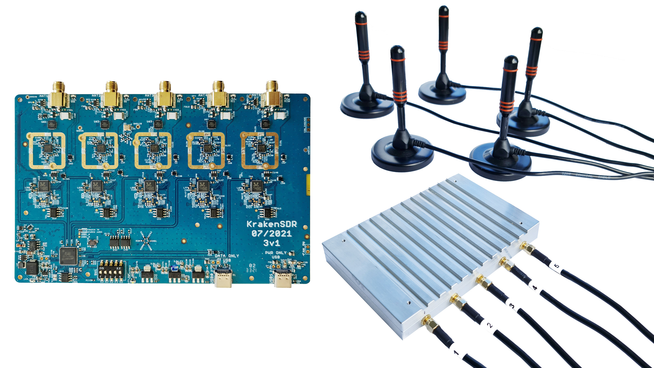
As discussed, analog phased arrays involve an analog phase shifter (and usually adjustable gain) per channel, meaning an analog phased array is a dedicated piece of hardware that must go alongside an SDR. On the other hand, any SDR that contains more than one channel can be used as a digital array with no extra hardware, as long as the channels are phase coherent and sampled using the same clock, which is typically the case for SDRs that have multiple recieve channels onboard. There are many SDRs that contain two receive channels, such as the Ettus USRP B210 and Analog Devices Pluto (the 2nd channel is exposed using a uFL connector on the board itself). Unfortunately, going beyond two channels involves entering the $10k+ segment of SDRs, at least as of 2023, such as the USRP N310. The main problem is that low-cost SDRs are typically not able to be “chained” together to scale the number of channels. The exception is the KerberosSDR (4 channels) and KrakenSDR (5 channels) which use multiple RTL-SDRs sharing an LO to form a low-cost digital array; the downside being the very limited sample rate (up to 2.56 MHz) and tuning range (up to 1766 MHz). The KrakenSDR board and example antenna configuration is shown below.

In this chapter we don’t use any specific SDRs; instead we simulate the receiving of signals using Python, and then go through the DSP used to perform beamforming/DOA for ditital arrays.

Array Factor Math

To get to the fun part we have to get through a little bit of math, but the following section has been written so that the math is extremely simple and has diagrams to go along with it, only the most basic trig and exponential properties are used. It’s important to understand the basic math behind what we’ll do in Python to perform DOA.

Consider a 1D three-element uniformly spaced array:

In this example a signal is coming in from the right side, so it’s hitting the right-most element first. Let’s calculate the delay between when the signal hits that first element and when it reaches the next element. We can do this by forming the following trig problem, try to visualize how this triangle was formed from the diagram above. The segment highlighted in red represents the distance the signal has to travel after it has reached the first element, before it hits the next one.

If you recall SOH CAH TOA, in this case we are interested in the “adjacent” side and we have the length of the hypotenuse (), so we need to use a cosine:

We must solve for adjacent, as that is what will tell us how far the signal must travel between hitting the first and second element, so it becomes adjacent . Now there is a trig identity that lets us convert this to adjacent . This is just a distance though, we need to convert this to a time, using the speed of light: time elapsed [seconds]. This equation applies between any adjacent elements of our array, although we can multiply the whole thing by an integer to calculate between non-adjacent elements since they are uniformly spaced (we’ll do this later).

Now to connect this trig and speed of light math to the signal processing world. Let’s denote our transmit signal at baseband and it’s being transmitting at some carrier, , so the transmit signal is . Lets say this signal hits the first element at time , which means it hits the next element after [seconds] like we calculated above. This means the 2nd element receives:

recall that when you have a time shift, it is subtracted from the time argument.

When the receiver or SDR does the downconversion process to receive the signal, its essentially multiplying it by the carrier but in the reverse direction, so after doing downconversion the receiver sees:

Now we can do a little trick to simplify this even further; consider how when we sample a signal it can be modeled by substituting for where is sample period and is just 0, 1, 2, 3… Substituting this in we get . Well, is so much greater than that we can get rid of the first term and we are left with . If the sample rate ever gets fast enough to approach the speed of light over a tiny distance, we can revisit this, but remember that our sample rate only needs to be a bit larger than the signal of interest’s bandwidth.

Let’s keep going with this math but we’ll start representing things in discrete terms so that it will better resemble our Python code. The last equation can be represented as the following, let’s plug back in :

We’re almost done, but luckily there’s one more simplification we can make. Recall the relationship between center frequency and wavelength: or the form we’ll use: . Plugging this in we get:

In DOA what we like to do is represent , the distance between adjacent elements, as a fraction of wavelength (instead of meters), the most common value chosen for during the array design process is to use one half the wavelength. Regardless of what is, from this point on we’re going to represent as a fraction of wavelength instead of meters, making the equation and all our code simpler:

This is for adjacent elements, for the ’th element we just need to multiply times :

And we’re done! This equation above is what you’ll see in DOA papers and implementations everywhere! We typically call that exponential term the “array factor” (often denoted as ) and represent it as an array, a 1D array for a 1D antenna array, etc. In python is:

a = [np.exp(-2j*np.pi*d*0*np.sin(theta)), np.exp(-2j*np.pi*d*1*np.sin(theta)), np.exp(-2j*np.pi*d*2*np.sin(theta)), ...] # note the increasing k
# or
a = np.exp(-2j * np.pi * d * np.arange(Nr) * np.sin(theta)) # where Nr is the number of receive antenna elements

Note how element 0 results in a 1+0j (because ); this makes sense because everything above was relative to that first element, so it’s receiving the signal as-is without any relative phase shifts. This is purely how the math works out, in reality any element could be thought of as the reference, but as you’ll see in our math/code later on, what matters is the difference in phase/amplitude received between elements. It’s all relative.

Receiving a Signal

Let’s use the array factor concept to simulate a signal arriving at an array. For a transmit signal we’ll just use a tone for now:

import numpy as np
import matplotlib.pyplot as plt

sample_rate = 1e6
N = 10000 # number of samples to simulate

# Create a tone to act as the transmitter signal
t = np.arange(N)/sample_rate # time vector
f_tone = 0.02e6
tx = np.exp(2j * np.pi * f_tone * t)

Now let’s simulate an array consisting of three omnidirectional antennas in a line, with 1/2 wavelength between adjacent ones (a.k.a. “half-wavelength spacing”). We will simulate the transmitter’s signal arriving at this array at a certain angle, theta. Understanding the array factor a below is why we went through all that math above.

d = 0.5 # half wavelength spacing
Nr = 3
theta_degrees = 20 # direction of arrival (feel free to change this, it's arbitrary)
theta = theta_degrees / 180 * np.pi # convert to radians
a = np.exp(-2j * np.pi * d * np.arange(Nr) * np.sin(theta)) # array factor
print(a) # note that it's a 1x3, it's complex, and the first element is 1+0j

To apply the array factor we have to do a matrix multiplication of a and tx, so first let’s convert both to matrices, as NumPy arrays which don’t let us do 1D matrix math that we need for beamforming/DOA. We then perform the matrix multiply, note that the @ symbol in Python means matrix multiply (it’s a NumPy thing). We also have to convert a from a row vector to a column vector (picture it rotating 90 degrees) so that the matrix multiply inner dimensions match.

a = np.asmatrix(a)
tx = np.asmatrix(tx)

r = a.T @ tx  # don't get too caught up by the transpose a, the important thing is we're multiplying the array factor by the tx signal
print(r.shape) # r is now going to be a 2D array, 1D is time and 1D is the spatial dimension

At this point r is a 2D array, size 3 x 10000 because we have three array elements and 10000 samples simulated. We can pull out each individual signal and plot the first 200 samples, below we’ll plot the real part only, but there’s also an imaginary part, like any baseband signal. One annoying part of Python is having to switch to matrix type for matrix math, then having to switch back to normal NumPy arrays, we need to add the .squeeze() to get it back to a normal 1D NumPy array.

plt.plot(np.asarray(r[0,:]).squeeze().real[0:200]) # the asarray and squeeze are just annoyances we have to do because we came from a matrix
plt.plot(np.asarray(r[1,:]).squeeze().real[0:200])
plt.plot(np.asarray(r[2,:]).squeeze().real[0:200])
plt.show()

Note the phase shifts between elements like we expect to happen (unless the signal arrives at boresight in which case it will reach all elements at the same time and there wont be a shift, set theta to 0 to see). Element 0 appears to arrive first, with the others slightly delayed. Try adjusting the angle and see what happens.

One thing we didn’t bother doing yet- let’s add noise to this received signal. AWGN with a phase shift applied is still AWGN, and we want to apply the noise after the array factor is applied, because each element experiences an independent noise signal.

n = np.random.randn(Nr, N) + 1j*np.random.randn(Nr, N)
r = r + 0.1*n # r and n are both 3x10000

Basic DOA

So far this has been simulating the receiving of a signal from a certain angle of arrival. In your typical DOA problem you are given samples and have to estimate the angle of arrival(s). There are also problems where you have multiple received signals from different directions and one is the signal-of-interest (SOI) while another might be a jammer or interferer you have to null out to extract the SOI with at as high SNR as possible.

Next let’s use this signal r but pretend we don’t know which direction the signal is coming in from, let’s try to figure it out with DSP and some Python code! We’ll start with the “conventional” beamforming approach, which involves scanning through (sampling) all directions of arrival from -pi to +pi (-180 to +180 degrees). At each direction we point the array towards that angle by applying the weights associated with pointing in that direction; applying the weights will give us a 1D array of samples, as if we received it with 1 directional antenna. You’re probably starting to realize where the term electrically steered array comes in. This conventional beamforming method involves calculating the mean of the magnitude squared, as if we were making an energy detector. We’ll apply the beamforming weights and do this calculation at a ton of different angles, so that we can check which angle gave us the max energy.

theta_scan = np.linspace(-1*np.pi, np.pi, 1000) # 1000 different thetas between -180 and +180 degrees
results = []
for theta_i in theta_scan:
    #print(theta_i)
    w = np.asmatrix(np.exp(-2j * np.pi * d * np.arange(Nr) * np.sin(theta_i))) # look familiar?
    r_weighted = np.conj(w) @ r # apply our weights corresponding to the direction theta_i
    r_weighted = np.asarray(r_weighted).squeeze() # get it back to a normal 1d numpy array
    results.append(np.mean(np.abs(r_weighted)**2)) # energy detector

# print angle that gave us the max value
print(theta_scan[np.argmax(results)] * 180 / np.pi) # 19.99999999999998

plt.plot(theta_scan*180/np.pi, results) # lets plot angle in degrees
plt.xlabel("Theta [Degrees]")
plt.ylabel("DOA Metric")
plt.grid()
plt.show()

We found our signal! Try increasing the amount of noise to push it to its limit, you might need to simulate more samples being received for low SNRs. Also try changing the direction of arrival.

If you prefer viewing angle on a polar plot, use the following code:

fig, ax = plt.subplots(subplot_kw={'projection': 'polar'})
ax.plot(theta_scan, results) # MAKE SURE TO USE RADIAN FOR POLAR
ax.set_theta_zero_location('N') # make 0 degrees point up
ax.set_theta_direction(-1) # increase clockwise
ax.set_rgrids([0,2,4,6,8])
ax.set_rlabel_position(22.5)  # Move grid labels away from other labels
plt.show()

180 Degree Ambiguity

Let’s talk about why is there a second peak at 160 degrees; the DOA we simulated was 20 degrees, but it is not a coincidence that 180 - 20 = 160. Picture three omnidirectional antennas in a line placed on a table. The array’s boresight is 90 degrees to the axis of the array, as labeled in the first diagram in this chapter. Now imagine the transmitter in front of the antennas, also on the (very large) table, such that its signal arrives at a +20 degree angle from boresight. Well the array sees the same effect whether the signal is arriving with respect to its front or back, the phase delay is the same, as depicted below with the array elements in red and the two possible transmitter DOA’s in green. Therefore, when we perform the DOA algorithm, there will always be a 180 degree ambiguity like this, the only way around it is to have a 2D array, or a second 1D array positioned at any other angle w.r.t the first array. You may be wondering if this means we might as well only calculate -90 to +90 degrees to save compute cycles, and you would be correct!

Broadside of the Array

To demonstrate this next concept, let’s try sweeping the angle of arrival (AoA) from -90 to +90 degrees instead of keeping it constant at 20:

As we approach the broadside of the array (a.k.a. endfire), which is when the signal arrives at or near the axis of the array, performance drops. We see two main degradations: 1) the main lobe gets wider and 2) we get ambiguity and don’t know whether the signal is coming from the left or the right. This ambiguity adds to the 180 degree ambiguity discussed earlier, where we get an extra lobe at 180 - theta, causing certain AoA to lead to three lobes of roughly equal size. This broadside ambiguity makes sense though, the phase shifts that occur between elements are identical whether the signal arrives from the left or right side w.r.t. the array axis. Just like with the 180 degree ambiguity, the solution is to use a 2D array or two 1D arrays at different angles. In general, beamforming works best when the angle is closer to the boresight.

When d is not λ/2

So far we have been using a distance between elements, d, equal to one half wavelength. So for example, an array designed for 2.4 GHz WiFi with λ/2 spacing would have a spacing of 3e8/2.4e9/2 = 12.5cm or about 5 inches, meaning a 4x4 element array would be about 15” x 15” x the height of the antennas. There are times when an array may not be able to achieve exactly λ/2 spacing, such as when space is restricted, or when the same array has to work on a variety of carrier frequencies.

Let’s examine when the spacing is greater than λ/2, i.e., too much spacing, by varying d between λ/2 and 4λ. We will remove the bottom half of the polar plot since it’s a mirror of the top anyway.

As you can see, in addition to the 180 degree ambiguity we discussed earlier, we now have additional ambiguity, and it gets worse as d gets higher (extra/incorrect lobes form). These extra lobes are known as grating lobes, and they are a result of “spatial aliasing”. As we learned in the IQ Sampling chapter, when we don’t sample fast enough we get aliasing. The same thing happens in the spatial domain; if our elements are not spaced close enough together w.r.t. the carrier frequency of the signal being observed, we get garbage results in our analysis. You can think of spacing out antennas as sampling space! In this example we can see that the grating lobes don’t get too problematic until d > λ, but they will occur as soon as you go above λ/2 spacing.

Now what happens when d is less than λ/2, such as when we need to fit the array in a small space? Let’s repeat the same simulation:

While the main lobe gets wider as d gets lower, it still has a maximum at 20 degrees, and there are no grating lobes, so in theory this would still work (at least at high SNR). To better understand what breaks as d gets too small, let’s repeat the experiment but with an additional signal arriving from -40 degrees:

Once we get lower than λ/4 there is no distinguishing between the two different paths, and the array performs poorly. As we will see later in this chapter, there are beamforming techniques that provide more precise beams than conventional beamforming, but keeping d as close to λ/2 as possible will continue to be a theme.

Antennas

Coming soon!

• common antenna types used for arrays (eg patch, monopole)

Number of Elements

Coming soon!

Capon’s Beamformer

In the basic DOA example we swept across all angles, multiplying r by the weights w, applying an energy detector to the resulting 1D array. In that example, w was equal to the array factor, a, so we were essentially just multiplying r by a. We will now look at a beamformer that is slightly more complicated but tends to perform much better, called Capon’s Beamformer, a.k.a. the minimum variance distortionless response (MVDR) beamformer. This beamformer can be summarized in the following equation:

where is the sample covariance matrix, calculated by multiplying r with the complex conjugate transpose of itself, , and the result will be a Nr x Nr size matrix (3x3 in the examples we have seen so far). This covariance matrix tells us how similar the samples received from the three elements are, although to use Capon’s method we don’t have to fully understand how that works. In textbooks and other resources you might see the Capon’s equation with some terms in the numerator; these are purely for scaling/normalization and they don’t change the results.

We can implement the equations above in Python fairly easily:

theta_scan = np.linspace(-1*np.pi, np.pi, 1000) # between -180 and +180 degrees
results = []
for theta_i in theta_scan:
    a = np.asmatrix(np.exp(-2j * np.pi * d * np.arange(Nr) * np.sin(theta_i))) # array factor
    a = a.T # needs to be a column vector for the math below

    # Calc covariance matrix
    R = r @ r.H # gives a Nr x Nr covariance matrix of the samples

    Rinv = np.linalg.pinv(R) # pseudo-inverse tends to work better than a true inverse

    metric = 1/(a.H @ Rinv @ a) # Capon's method!
    metric = metric[0,0] # convert the 1x1 matrix to a Python scalar, it's still complex though
    metric = np.abs(metric) # take magnitude
    metric = 10*np.log10(metric) # convert to dB so its easier to see small and large lobes at the same time
    results.append(metric)

results /= np.max(results) # normalize

When applied to the previous DOA example code, we get the following:

Works fine, but to really compare this to other techniques we’ll have to create a more interesting problem. Let’s set up a simulation with an 8-element array receiving three signals from different angles: 20, 25, and 40 degrees, with the 40 degree one received at a much lower power than the other two. Our goal will be to detect all three. The code to generate this new scenario is as follows:

Nr = 8 # 8 elements
theta1 = 20 / 180 * np.pi # convert to radians
theta2 = 25 / 180 * np.pi
theta3 = -40 / 180 * np.pi
a1 = np.asmatrix(np.exp(-2j * np.pi * d * np.arange(Nr) * np.sin(theta1)))
a2 = np.asmatrix(np.exp(-2j * np.pi * d * np.arange(Nr) * np.sin(theta2)))
a3 = np.asmatrix(np.exp(-2j * np.pi * d * np.arange(Nr) * np.sin(theta3)))
# we'll use 3 different frequencies
r = a1.T @ np.asmatrix(np.exp(2j*np.pi*0.01e6*t)) + \
    a2.T @ np.asmatrix(np.exp(2j*np.pi*0.02e6*t)) + \
    0.1 * a3.T @ np.asmatrix(np.exp(2j*np.pi*0.03e6*t))
n = np.random.randn(Nr, N) + 1j*np.random.randn(Nr, N)
r = r + 0.04*n

And if we run our Capon’s beamformer on this new scenario we get the following results:

It works pretty well, we can see the two signals received only 5 degrees apart, and we can also see the 3rd signal (at -40 or 320 degrees) that was received at one tenth the power of the others. Now let’s run the simple beamformer which is just an energy detector on this new scenario:

While it might be a pretty shape, it’s not finding all three signals at all… By comparing these two results we can see the benefit from using a more complex beamformer. There are many more beamformers out there, but next we are going to dive into a different class of beamformer that use the “subspace” method, often called adaptive beamforming.

MUSIC

We will now change gears and talk about a different kind of beamformer. All of the previous ones have fallen in the “delay-and-sum” category, but now we will dive into “sub-space” methods. These involve dividing the signal subspace and noise subspace, which means we must estimate how many signals are being received by the array, to get a good result. MUltiple SIgnal Classification (MUSIC) is a very popular sub-space method that involves calculating the eigenvectors of the covariance matrix (which is a computationally intensive operation by the way). We split the eigenvectors into two groups: signal sub-space and noise-subspace, then project steering vectors into the noise sub-space and steer for nulls. That might seem confusing at first, which is part of why MUSIC seems like black magic!

The core MUSIC equation is the following:

where is that list of noise sub-space eigenvectors we mentioned (a 2D matrix). It is found by first calculating the eigenvectors of , which is done simply by w, v = np.linalg.eig(R) in Python, and then splitting up the vectors (w) based on how many signals we think the array is receiving. There is a trick for estimating the number of signals that we’ll talk about later, but it must be between 1 and Nr - 1. I.e., if you are designing an array, when you are choosing the number of elements you must have one more than the number of anticipated signals. One thing to note about the equation above is does not depend on the array factor , so we can precalculate it before we start looping through theta. The full MUSIC code is as follows:

num_expected_signals = 3 # Try changing this!

# part that doesn't change with theta_i
R = r @ r.H # Calc covariance matrix, it's Nr x Nr
w, v = np.linalg.eig(R) # eigenvalue decomposition, v[:,i] is the eigenvector corresponding to the eigenvalue w[i]
eig_val_order = np.argsort(np.abs(w)) # find order of magnitude of eigenvalues
v = v[:, eig_val_order] # sort eigenvectors using this order
# We make a new eigenvector matrix representing the "noise subspace", it's just the rest of the eigenvalues
V = np.asmatrix(np.zeros((Nr, Nr - num_expected_signals), dtype=np.complex64))
for i in range(Nr - num_expected_signals):
   V[:, i] = v[:, i]

theta_scan = np.linspace(-1*np.pi, np.pi, 1000) # -180 to +180 degrees
results = []
for theta_i in theta_scan:
    a = np.asmatrix(np.exp(-2j * np.pi * d * np.arange(Nr) * np.sin(theta_i))) # array factor
    a = a.T
    metric = 1 / (a.H @ V @ V.H @ a) # The main MUSIC equation
    metric = np.abs(metric[0,0]) # take magnitude
    metric = 10*np.log10(metric) # convert to dB
    results.append(metric)

results /= np.max(results) # normalize

Running this algorithm on the complex scenario we have been using, we get the following very precise results, showing the power of MUSIC:

Now what if we had no idea how many signals were present? Well there is a trick; you sort the eigenvalue magnitudes from highest to lowest, and plot them (it may help to plot them in dB):

plot(10*np.log10(np.abs(w)),'.-')

The eigenvalues associated with the noise-subspace are going to be the smallest, and they will all tend around the same value, so we can treat these low values like a “noise floor”, and any eigenvalue above the noise floor represents a signal. Here we can clearly see there are three signals being received, and adjust our MUSIC algorithm accordingly. If you don’t have a lot of IQ samples to process or the signals are at low SNR, the number of signals might not be as obvious. Feel free to play around by adjusting num_expected_signals between 1 and 7, you’ll find that underestimating the number will lead to missing signal(s) while overestimating will only slightly hurt performance.

Another experiment worth trying with MUSIC is to see how close two signals can arrive at (in angle) while still distinguishing between them; sub-space techniques are especially good at that. The animation below shows an example, with one signal at 18 degrees and another slowly sweeping angle of arrival.

ESPRIT

Coming soon!

2D DOA

Coming soon!

Steering Nulls

Coming soon!

Conclusion and References

All Python code, including code used to generate the figures/animations, can be found on the textbook’s GitHub page.

• DOA implementation in GNU Radio - https://github.com/EttusResearch/gr-doa
• DOA implementation used by KrakenSDR - https://github.com/krakenrf/krakensdr_doa/blob/main/_signal_processing/krakenSDR_signal_processor.py